
Introduction
In this article, we will be discussing the Uniform Cost Search algorithm for finding the shortest route in a weighted graph. Uniform-Cost Search is one of the best algorithm for solving search problem that doesn’t require the use of Heuristics. It is able to deal with any common graph for the most efficient cost. Uniform Cost Search as it implies searches across branches that are roughly the same in cost.
Heuristics Search Techniques
A heuristic method of search is a form of search which tries to identify a feasible solution, but not always an ideal one, from the list of all the options available. The method makes decisions by weighing every option available for each part of a search. It then selects the most suitable option from the options that are presented. Instead of focusing on finding the most effective solution as other methods of searching, heuristic searches are created to be swift and hence determines the best alternative within a reasonable and within the allotted memory space.
Search Problem Statement
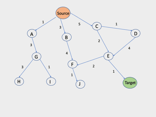
Let’s say we have an graph connecting all cities, which contains V nodes. Furthermore, we also have E edges that join the nodes. Each of these edges is assigned the weight which represents the cost to make use of the edge. There are two nodes which represent the source node in addition to the one that represents the final destination or target node respectively.
Our job is to discover the route starting from source S to Target T where we want to go using the standard costs search algorithm.
Uniform Cost Search
Uniform-Cost Search again demands the use of priority queues. The priority queue utilised here is similar to the prioritisation being given to the sum of the costs all the way up to that particular node. In contrast to Depth First Search where the highest depth was given the top importance, Uniform-Cost Search gives the cost with the least cumulative value with the highest priority. Uniform cost search is equivalent to BFS algorithm if the path cost of all edges is the same. The algorithm that uses this priority queue is as follows:
Algorithm
Add the root in the queueWhile Queue isn't emptyDequeue the highest priority element of the queue (If priorities are the same, an alphabetically smaller element will be taken)If the elements is the destination elementPrint the path and exit
ElseInsert all child of dequeued element using the sum of the costs prioritising the cumulative costs.
Lets apply this algorithm on above graph to find minimum shortest path between source and target.
Iteration 0
First, we will insert source node in the priority queue.

Visited Set: Source
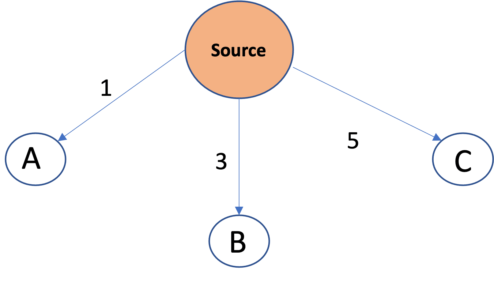
Iteration 1
Int the next iteration, we add source node’s children i.e A,B,C to the priority queue with their cumulative distance as priority:
Visited Set: Source
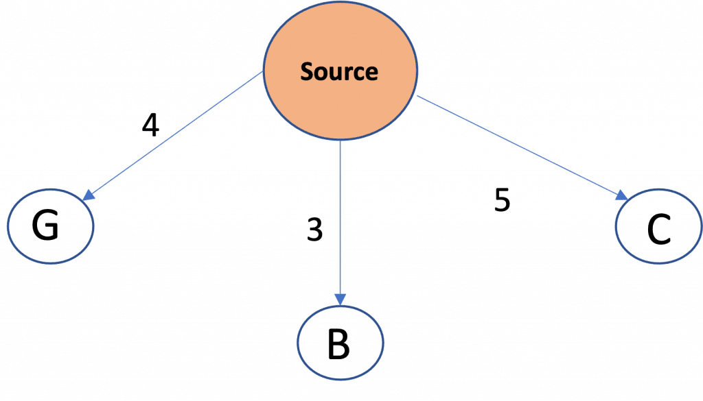
Iteration 2
Now, Since node A has the minimum distance / maximum priority , so it is fetched from the queue and added to visited set. And since A is not the destination, its children i.e G are added to the queue with their cumulative distance i.e 4 as priority (Source-> A-> G).
Visited Set: Source, A
Iteration 3
Node B has the minimum distance now, so its children i.e node F are added to the queue.

Visited Set: Source, A, B
Iteration 4
Up next, Node G will be removed and its children will be added to the queue likewise and visited set will be updated.
Visited Set: Source, A, B, G
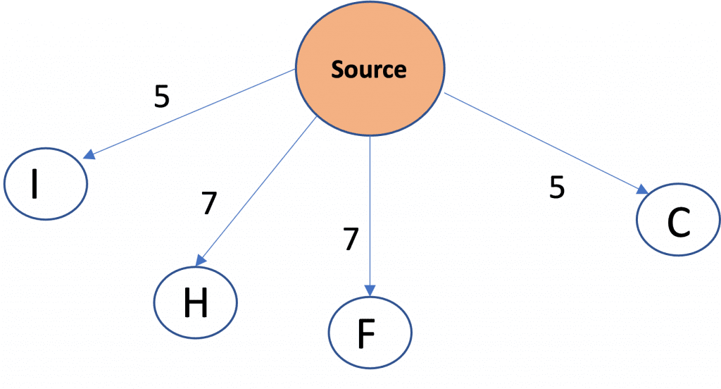
Iteration 5
Now, Since Node C and I have the same distance, so we will pick node alphabetically and add its children as done earlier.
Visited Set: Source, A, B, G, C
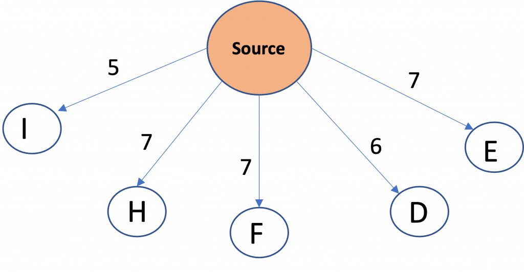
Iteration 6
Next, node I has minimum distance; however, node I has no further children, so queue will remain unchanged. After that, we remove D as D has next minimum distance.
Visited Set: Source, A, B, G, C, I
Iteration 7
D only has one child, E, with a cumulative distance of 10. But, we already have node E in our queue with a lesser distance, so we will not add it again.
Visited Set: Source, A, B, G, C, I, D
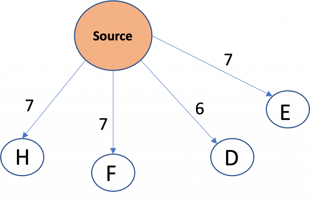
Iteration 8
The next minimum distance is that of E, so that will be processed further in similar way as done earlier
Visited Set: Source, A, B, G, C, I, D, E
Iteration 9
Now, the minimum cost is that of Node F, so it will be removed and its child i.e Node J will be pushed to priority queue.

Visited Set: Source, A, B, G, C, I, D, E, F
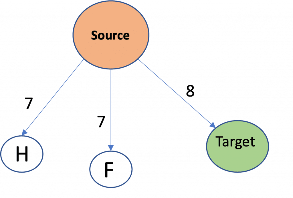
Iteration 10
Next, Node H has the minimum cost so it will be removed, but since it has no children no updation will be done.
Visited Set: Source, A, B, G, C, I, D, E, F, Target
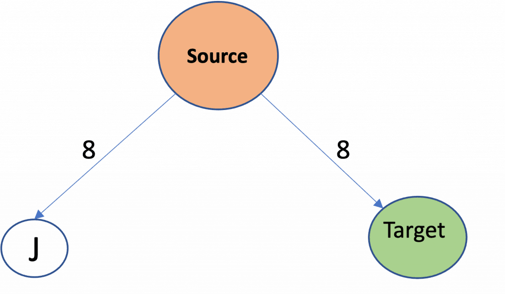
Iteration 11
Lastly, we have the Target node with next minimum distance and since its our destination node we will stop the algorithm here.
The minimum distance between the source and destination nodes is therefore 8.
KeyPoints
At any time during the execution process, the ucs algorithm does not expand an element that is more expensive than the price of the shortest path within the graph. The elements of the priority queue share the same cost at a moment in time, hence they are referred to as Uniform Cost Search.
Completeness:
The search for uniform cost search algorithm is complete in that If there’s any solution, UCS will find it.
Time Complexity:
Let C* be the cost for the best solution and t is the step to be closer to the desired node. The number of steps is 1+ C*/t. In this case, we’ve taken one more step, starting at state 0 and work our way to C*/t.
Therefore, the maximum time complexity of a search using Uniform-cost is O(b1 + [C*/t])
Space Complexity:
The same principle applies for space complexity , so the space complexity in the worst-case scenario of Uniform-cost Search would be O(b1 + [C*/t]).
Optimal:
The search for uniform cost is always the best since it selects only one path that is the least expensive cost for the path.
Advantages
- It is helpful to identify the route with the lowest cost per mile within the weighted graph that has an individual cost for every edge that runs from the node at the beginning to that node.
- It is thought to be the most optimal solution as, at every point, the most efficient route is thought to follow.
Disadvantage
- The list has to be sorted in accordance with the priority queue has to be kept.
- The amount of storage needed is enormous.
- The ucs algorithm could be stuck in an endless loop because it takes into account all possible routes from the node at the beginning to your destination point.
Conclusion
Uniform-Cost Search is a form of search algorithm that is uninformed and the best solution to determine the best route from the root node to destination with the lowest total cost in a search space that is weighted in which each node is characterised by an individual cost of traversal.
Got a question or just want to chat? Comment below or drop by our forums, where a bunch of the friendliest people you’ll ever run into will be happy to help you out!