Asymptotic Notations are used to describe the performance of algorithms. It specifically describes how fast the runtime grows relative to the input size.
Let’s think about searching for a name in a phone book as an example. If the phone book had 10 names, it might take 1 second to find a name compared to 1,000, which might take 60 seconds. See how the time is growing as the phone book gets bigger? Asymptotic Notations formalize this growth rate.
Asymptotic Notations are like speedometers for algorithms. Just as a speedometer shows how fast a car is going, these notations give us an idea of how fast or slow an algorithm runs, especially when dealing with a lot of data. Instead of getting lost in detailed steps of the algorithm, we use these notations to get a bird’s-eye view of its performance.
Types of Asymptotic Notations:
- Big O Notation (O)
- Omega Notation (Ω)
- Theta Notation (Θ)
- Little o Notation (o)
- Little omega Notation (ω)
In this article we will mainly focus on understanding Big O Notation with examples. So, let’s get started.
What is Big O Notation In Data Structure?
Big O notation in data structure describes the upper bound on an algorithm’s runtime. It tells you the worst-case scenario on how long an algorithm will take to run.
For example, let’s say you had an algorithm with a runtime of O(n). This means its worst-case runtime grows linearly with the size of the input. So if n is the number of elements:
- If n is 10, the algorithm might take at most 10 seconds.
- If n is 100, the algorithm might take at most 100 seconds.
- If n is 1000, the algorithm might take at most 1000 seconds.
The key word here is “might“. Big O only tells you the upper bound, which means the algorithm will take at most that much time. The actual runtime could be better! For that O(n) algorithm:
- If n is 10, the algorithm could run in 5 seconds.
- If n is 100, the algorithm could run in 50 seconds.
Because Big O describes the worst case, the actual runtime will be the same or better. Big O Notation gives you a guarantee on the maximum time, but the algorithm could do better. Big O is useful when comparing algorithms. You can use Big O to understand which algorithm will perform better as the input grows, even without knowing the exact runtimes.
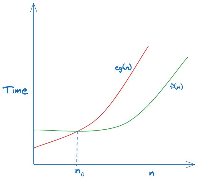
Formal Definition Of Big O Notation
Let f(n) and g(n) be two functions defined on the positive integers. We say that f(n) is O(g(n)) if there exist constants c > 0 and n0 > 0 such that for all n >= n0:
f(n) <= c * g(n)
This means there is some constant factor c such that f grows no faster than cg(n) for sufficiently large n. The formal definition requires f to be asymptotically bounded above by cg(n).
So, Mathematical formula for Big O is
O(g(n)) = { f(n): there exist positive constants c and n0 such that 0 <= f(n) <= cg(n) for all n >= n0 }
Intuitively, f(n) = O(g(n)) means that g(n) provides an upper bound on the growth rate of f(n). As n increases, f(n) grows no faster than g(n) up to constant factors.
How To Calculate Time Complexity With Big O Notation?
Let’s now see steps on how we can calculate Time Complexity with Big O Notation of given algorithm:
Steps To Calculate Time Complexity With Big O Notation are:
int minOperations(int[] arr) {
  int count = 0;

  for (int i = 0; i < arr.length; i++) {
    for (int j = i+1; j < arr.length; j++) {
      if (arr[i] > arr[j]) {
        int temp = arr[i];
        arr[i] = arr[j];
        arr[j] = temp;
        count++;
      }
    }
  }

  return count;
}
1. Assume the worst case: Since Big O is the worst-case scenario for any algorithm, always consider the maximum number of operations that could be executed for any input. For example, for loops, assume they iterate fully through the end condition, and for recursive functions, assume the maximum recursion depth. For example:
For the above code example, the array length is ‘l.’ Considering worst-case scenarios. The outer loop will run l times, and the inner loop will l*(l-1)/2 times (l + (l-1) + (l-2) …. 1 ). Considering if the statement is always true. The swap operation will run, therefore, l*(l-1)/2 times.
2. Remove constants: The number of operations doesn’t matter; only the growth rate matters. Therefore, omit any constant factors in the operation count. This simplifies the expression to focus just on the growth.
3. Use different terms for inputs: Substitute simple variable names for input parameters. Generally, n is often substituted for the size of a data structure like array length. This allows generalizing beyond the specific input values.
So, for the above example, the arraylength can be substituted with n. Therefore, the swap operation will run therefore n*(n-1)/2 times
4. Drop non-dominant terms: Focus only on the fastest growing component w.r.t. input and drop any lower order terms as n increases. This keeps only the most significant term for large n.
So in above example n*(n-1)/2 dominates the growth
Therefore Time Complexity for the above code is O(n*(n-1)/2) ≈ O(n2).
Master theorem can also be used to solve time complexity of recurrence relations of the form:
T(n) = aT(n/b) + f(n)
How To Calculate Space Complexity With Big O Notation?
void duplicateArray(int[] arr) {
  int n = arr.length;
  int[] copy = new int[n]; // Allocate new array

  for (int i = 0; i < n; i++) {
    copy[i] = arr[i];
  }
}
Let’s now see the steps on how we can calculate Space Complexity with the Big O Notation of the given algorithm:
1. Determine all storage used by the algorithm: Determine all input and output data structures like arrays or strings created, Variables/references used for storing values, Program stack space for recursion, etc. For the above code example, we have one variable n to store array length, one copy array, and one input array.
2. Assume the worst case for dynamic memory allocation: Assume Arrays or collections are max sizes, and recursion has maximum depth. Considering the worst case, the copy array is max allocated to the array length.
3. Remove constants: Since Big O is an approximation focusing only on growth as the input size increases, exact storage sizes don’t matter. So, space complexity 2Arraylength ==> Arraylength
4. Use different terms for input sizes: Substitute variable names for input parameters. The general convention is to use ‘n’. Replacing Arraylength with n for the above code example, space complexity can be denoted as O(n).
5. Focus on dominant storage: Look at space usage that grows fastest with input size. For the above example, the Output array dominates, growing as n
Space Complexity for the above code is, therefore, O(n).
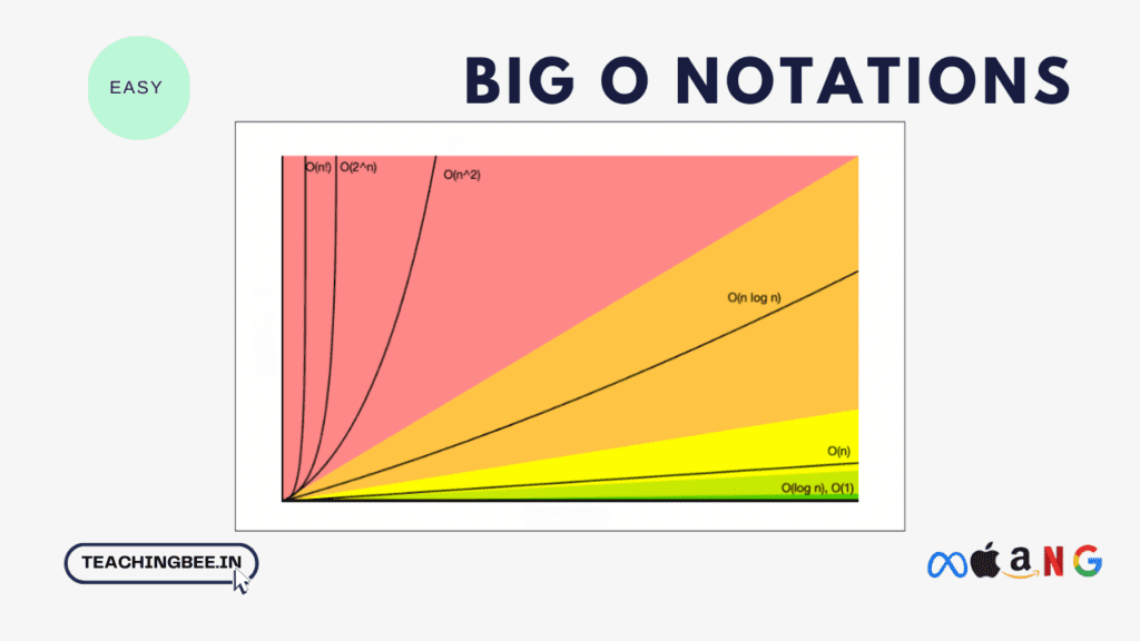
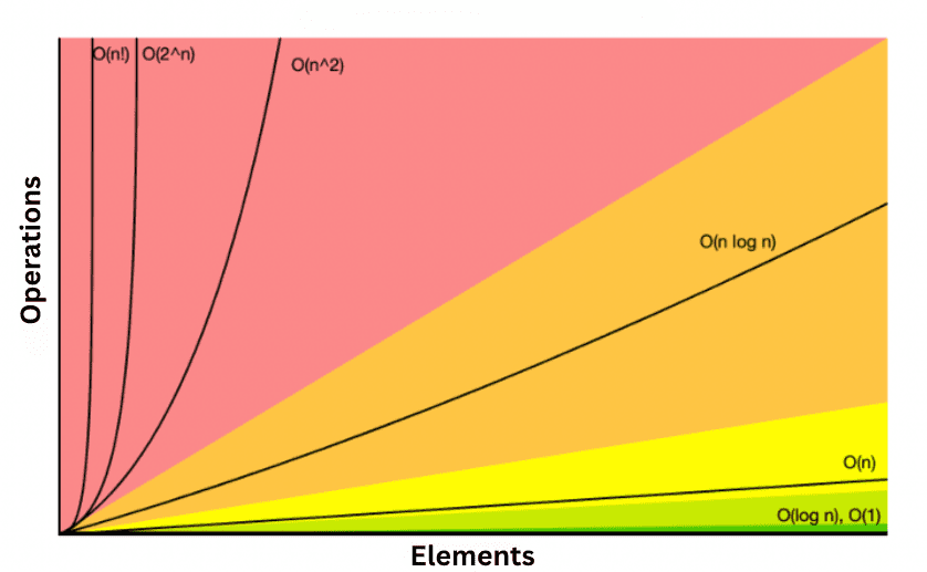
Big O Notation With Examples
The most common Big O notations and their time complexities are
| Big O Notation | Name | Description | Example |
|---|---|---|---|
| O(1) | Constant time | Runtime is constant regardless of input size. | Accessing array element by index |
| O(log n) | Logarithmic time | Doubling input size increases runtime by a constant amount. | Binary search on sorted array |
| O(n) | Linear time | Doubling input size doubles the runtime. | Sequential search on array |
| O(n log n) | Log-linear time | Doubling input increases runtime by a log n factor. | Efficient sorting algorithms |
| O(n^2) | Quadratic time | Doubling input size quadruples the runtime. | Nested loops |
| O(n^3) | Cubic time | Doubling input size increases runtime by 8x. | Triple nested loops |
| O(2^n) | Exponential time | Doubling input size doubles the exponent. | Recursive Fibonacci |
| O(n!) | Factorial time | Runtime grows enormously even for small inputs. | Brute force TSP |
| O(n^c) | Polynomial time | Grows faster than linear but slower than exponential. | Matrix multiplication |
| O(c^n) | Exponential time | Grows extremely fast, even faster than 2^n. | Combinatorics |
| O(n log n) | Quasilinear time | In between linear and quadratic time. | Fast Fourier Transform |
Let’s see some of the code examples of these Big O notation
O(1) – Constant Time
// Accessing the element in array.
int get_element(int arr[], int index) {
    return arr[index];
}
The above code has constant time complexity as no matter how large the input size grows, accessing an element in array using index always takes a constant amount of time.
O(log n) – Logarithmic Time
// Binary Search

int binary_search(int arr[], int size, int x) {
    int low = 0;
    int high = size - 1;
    while (low <= high) {
        int mid = (low + high) / 2;
        if (arr[mid] == x) {
            return mid;
        } else if (arr[mid] < x) {
            low = mid + 1;
        } else {
            high = mid - 1;
        }
    }
    return -1;
}
The above is for binary search. Binary search works by repeatedly dividing the search interval in half. Repeatedly, the interval is halved until it narrows down to the desired value or becomes empty.So, while loop is executed for log(n) times..For detailed explanation you can see this.
O(n) – Linear Time
// Linear search

int linear_search(int arr[], int size, int x) {
    for (int i = 0; i < size; i++) {
        if (arr[i] == x) {
            return i;
        }
    }
    return -1;
}
The linear search algorithm works by iterating through each element of the array one by one until it finds the desired value or reaches the end of the array. The worst case scenario will be that the desired value is the last element of the array or not in the array at all. In this case, n comparisons are made, where n is the size of the array.So time complexity is O(n).
O(n log n) – Log-linear Time
// Merge Sort

// Merge two subarrays of arr[]
// First subarray is arr[l..m]
// Second subarray is arr[m+1..r]
void merge(int arr[], int l, int m, int r) {
    int i, j, k;
    int n1 = m - l + 1;
    int n2 = r - m;

    // Create temporary arrays
    int L[n1], R[n2];

    // Copy data to temporary arrays L[] and R[]
    for (i = 0; i < n1; i++)
        L[i] = arr[l + i];
    for (j = 0; j < n2; j++)
        R[j] = arr[m + 1 + j];

    // Merge the temporary arrays back into arr[l..r]
    i = 0; // Initial index of first subarray
    j = 0; // Initial index of second subarray
    k = l; // Initial index of merged subarray
    while (i < n1 && j < n2) {
        if (L[i] <= R[j]) {
            arr[k] = L[i];
            i++;
        } else {
            arr[k] = R[j];
            j++;
        }
        k++;
    }

    // Copy the remaining elements of L[], if there are any
    while (i < n1) {
        arr[k] = L[i];
        i++;
        k++;
    }

    // Copy the remaining elements of R[], if there are any
    while (j < n2) {
        arr[k] = R[j];
        j++;
        k++;
    }
}

// Main merge sort function
void mergeSort(int arr[], int l, int r) {
    if (l < r) {
        // Same as (l+r)/2, but avoids overflow for large l and r
        int m = l + (r - l) / 2;

        // Sort first and second halves
        mergeSort(arr, l, m);
        mergeSort(arr, m + 1, r);

        // Merge the sorted halves
        merge(arr, l, m, r);
    }
}
The code demonstrates the Merge Sort algorithm, which has a time complexity of O(n*log(n)). Here’s why:
- Merge Sort follows a divide-and-conquer strategy. It recursively divides the input array into two halves until each sub-array contains only one element. This division process takes O(log(n)) time because the array is continuously divided into halves.
- After the division, it performs merging operations. Merging two sorted arrays of size n/2 each takes O(n) time, as it involves comparing and combining all elements of both arrays. Since we perform this merging operation at each level of recursion, the total time spent on merging is O(n*log(n)).
O(2^n) – Exponential Time
// Fibonacci

// Recursive function to calculate Fibonacci numbers
int fibonacci(int n) {
    if (n <= 1) {
        return n;
    }
    return fibonacci(n - 1) + fibonacci(n - 2);
}
The recursive Fibonacci function has a branching factor of 2 at each level of recursion because it makes two recursive calls, one for fibonacci(n - 1) and one for fibonacci(n - 2). This means that at each level, the number of function calls doubles. As a result, the total number of function calls grows exponentially with the input n.
Big O Notation Practice Problems
Let’s test the knowledge with some practice questions.
Q1. What is the time, and space complexity of the following code?
#include <stdio.h>

int main() {
    int n = 16; // Replace with your desired value of n
    int i, j, k = 0;

    for (i = n / 2; i <= n; i++) {
        for (j = 2; j <= n; j = j * 2) {
            k = k + n / 2;
        }
    }

    printf("Result (k): %d\n", k);
    return 0;
}
Answer: Time Complexity: O(n log n) Space Complexity: O(1)
Q2. What is the time, and space complexity of the following code?
#include <stdio.h>

int main() {
    int N = 16; // Replace with your desired value of N
    int a = 0, i = N;

    while (i > 0) {
        a += i;
        i /= 2;
    }

    printf("Result (a): %d\n", a);
    return 0;
}
Answer: Time Complexity: O(log n) Space Complexity: O(1)
Q3. What is the time, and space complexity of the following code?
#include <stdio.h>

int main() {
    int n = 5; // Replace with your desired value of n
    int value = 0;

    for (int i = 0; i < n; i++) {
        for (int j = 0; j < i; j++) {
            value += 1;
        }
    }

    printf("Result (value): %d\n", value);
    return 0;
}
Answer: Time Complexity: O(n^2) Space Complexity: O(1)
Key TakeAways
To conclude:
- Asymptotic notations like Big O are used to describe the performance of algorithms, specifically the growth rate of runtime related to input size.
- Big O notation provides an asymptotic upper bound on the worst case runtime of an algorithm, expressed in terms of input size n.
- The formal definition of Big O is that f(n) = O(g(n)) if f(n) grows no faster than g(n) asymptotically, up to constant factors.
- Calculating Big O involves determining the fastest growing operation in an algorithm, simplifying with rules like dropping constants and non-dominant terms.
- Common Big O runtimes include O(1), O(log n), O(n), O(n log n), O(n^2), O(2^n) etc based on growth rates like constant, logarithmic, linear, quadratic, exponential.
Checkout more C Tutorials here.
I hope You liked the post ?. For more such posts, ? subscribe to our newsletter. Try out our free resume checker service where our Industry Experts will help you by providing resume score based on the key criteria that recruiters and hiring managers are looking for.
FAQ
What are properties of Big O Notation ?
Key Properties of Big O Notation
- Reflexivity: For any function f(n), f(n) = O(f(n)). The function describes an upper bound for itself.
- Transitivity: If f(n) = O(g(n)) and g(n) = O(h(n)), then f(n) = O(h(n)). Transitivity allows extending upper bound relationships.
- Symmetry: If f(n) = O(g(n)), then g(n) = O(f(n)). The upper bound relationship works symmetrically in both directions.
- Transpose Symmetry: If f(n) = O(g(n)), then af(n) + b = O(g(n)) for constants a > 0, b. Shifting/scaling by constants doesn’t affect asymptotic upper bound.
- Subadditivity: If f(n) = O(h(n)) and g(n) = O(p(n)), then f(n) + g(n) = O(h(n) + p(n)). Upper bounds on functions extend to their sum.
Why is Big O Notation important?
- Algorithm Classification: Big O notation classifies algorithms by their worst-case time complexity, aiding in algorithm selection and analysis.
- Platform Agnostic Comparisons: It abstracts away platform-specific details, allowing comparisons based solely on scalability.
- Algorithm Selection: Big O helps choose algorithms meeting performance constraints and informs tradeoffs.
- Foundation for Complexity Theory: It forms the basis for computational complexity theory, exploring algorithmic limitations and capabilities.